Continuous Coordinates#
HoloViews is designed to work with scientific and engineering data, which is often in the form of discrete samples from an underlying continuous system. Imaging data is one clear example: measurements taken at a regular interval over a grid covering a two-dimensional area. Although the measurements are discrete, they approximate a continuous distribution, and HoloViews provides extensive support for working naturally with data of this type.
2D Continuous spaces#
In this user guide we will show the support provided by HoloViews for working with two-dimensional regularly sampled grid data like images, and then in subsequent sections discuss how HoloViews supports one-dimensional, higher-dimensional, and irregularly sampled data with continuous coordinates.
import numpy as np

import holoviews as hv
from holoviews import opts

hv.extension('bokeh')

np.set_printoptions(precision=2, linewidth=80)
opts.defaults(opts.Layout(shared_axes=False))


First, let’s consider:
|
a simple function that accepts a location in a 2D plane specified in millimeters (mm) |
|
a 1mm×1mm square region of this 2D plane, centered at the origin, and |
|
a function returning a square (s×s) grid of (x,y) coordinates regularly sampling the region in the given bounds, at the centers of each grid cell |
def f(x,y):
    return x+y/3.1

region=(-0.5,-0.5,0.5,0.5)

def coords(bounds,samples):
    l,b,r,t=bounds
    hc=0.5/samples
    return np.meshgrid(np.linspace(l+hc,r-hc,samples),
                       np.linspace(b+hc,t-hc,samples))
Now let’s build a Numpy array regularly sampling this function at a density of 5 samples per mm:
f5=f(*coords(region,5))
f5
array([[-0.53, -0.33, -0.13,  0.07,  0.27],
       [-0.46, -0.26, -0.06,  0.14,  0.34],
       [-0.4 , -0.2 ,  0.  ,  0.2 ,  0.4 ],
       [-0.34, -0.14,  0.06,  0.26,  0.46],
       [-0.27, -0.07,  0.13,  0.33,  0.53]])
We can visualize this array (and thus the function f) either using a Raster, which uses the array’s own integer-based coordinate system (which we will call “array” coordinates), or an Image, which uses a continuous coordinate system, or as a HeatMap labelling each value explicitly:
r5 = hv.Raster(f5, label="R5")
i5 = hv.Image( f5, label="I5", bounds=region)
h5 = hv.HeatMap([(x, y, round(f5[4-y,x],2)) for x in range(5) for y in range(5)], label="H5")

h5_labels = hv.Labels(h5).opts(padding=0)

r5 + i5 + h5*h5_labels
Both the Raster and Image Element types accept the same input data and show the same arrangement of colors, but a visualization of the Raster type reveals the underlying raw array indexing, while the Image type has been labelled with the coordinate system from which we know the data has been sampled. All Image operations work with this continuous coordinate system instead, while the corresponding operations on a Raster use raw array indexing.
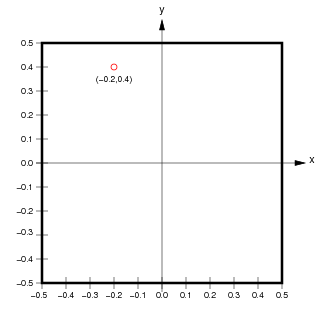
For instance, all five of these indexing operations refer to the same element of the underlying Numpy array, i.e. the second item in the first row:
f"{r5[0, 1] = :0.2f}, {r5.data[0, 1] = :0.2f}, {i5[-0.2, 0.4] = :0.2f}, {i5[-0.24, 0.37] = :0.2f}, {i5.data[0, 1] = :0.2f}"
'r5[0, 1] = -0.46, r5.data[0, 1] = -0.33, i5[-0.2, 0.4] = -0.33, i5[-0.24, 0.37] = -0.33, i5.data[0, 1] = -0.33'
You can see that the Raster and the underlying .data elements both use Numpy’s raw integer indexing, while the Image uses floating-point values that are then mapped onto the appropriate array element.
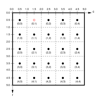
This diagram should help show the relationships between the Raster coordinate system in the plot (which ranges from 0 at the top edge to 5 at the bottom), the underlying raw Numpy integer array indexes (labelling each dot in the Array coordinates figure), and the underlying Continuous coordinates:
 |
 |
Importantly, although we used a 5×5 array in this example, we could substitute a much larger array with the same continuous coordinate system if we wished, without having to change any of our continuous indexes – they will still point to the correct location in the continuous space:
f10=f(*coords(region,10))
f10
array([[-0.6 , -0.5 , -0.4 , -0.3 , -0.2 , -0.1 ,  0.  ,  0.1 ,  0.2 ,  0.3 ],
       [-0.56, -0.46, -0.36, -0.26, -0.16, -0.06,  0.04,  0.14,  0.24,  0.34],
       [-0.53, -0.43, -0.33, -0.23, -0.13, -0.03,  0.07,  0.17,  0.27,  0.37],
       [-0.5 , -0.4 , -0.3 , -0.2 , -0.1 ,  0.  ,  0.1 ,  0.2 ,  0.3 ,  0.4 ],
       [-0.47, -0.37, -0.27, -0.17, -0.07,  0.03,  0.13,  0.23,  0.33,  0.43],
       [-0.43, -0.33, -0.23, -0.13, -0.03,  0.07,  0.17,  0.27,  0.37,  0.47],
       [-0.4 , -0.3 , -0.2 , -0.1 , -0.  ,  0.1 ,  0.2 ,  0.3 ,  0.4 ,  0.5 ],
       [-0.37, -0.27, -0.17, -0.07,  0.03,  0.13,  0.23,  0.33,  0.43,  0.53],
       [-0.34, -0.24, -0.14, -0.04,  0.06,  0.16,  0.26,  0.36,  0.46,  0.56],
       [-0.3 , -0.2 , -0.1 , -0.  ,  0.1 ,  0.2 ,  0.3 ,  0.4 ,  0.5 ,  0.6 ]])
r10 = hv.Raster(f10, label="R10")
i10 = hv.Image(f10, label="I10", bounds=region)
r10+i10
The image now has higher resolution, but still visualizes the same underlying continuous function, now evaluated at 100 grid positions instead of 25:
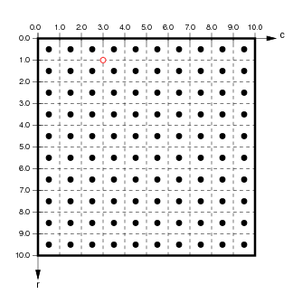 |
|
Indexing the exact same coordinates as above now gets very different results:
f"{r10[1, 0] = :0.2f}, {r10.data[0,1] = :0.2f}, {i10[-0.2, 0.4] = :0.2f}, {i10[-0.24, 0.37] = :0.2f} {i10.data[0, 1] = :0.2f}"
'r10[1, 0] = -0.50, r10.data[0,1] = -0.50, i10[-0.2, 0.4] = -0.30, i10[-0.24, 0.37] = -0.36 i10.data[0, 1] = -0.50'
The array-based indexes used by Raster and the Numpy array in .data still return the second item in the first row of the array, but this array element now corresponds to location (-0.35,0.4) in the continuous function, and so the value is different. These indexes thus do not refer to the same location in continuous space as they did for the other array density, because raw Numpy-based indexing is not independent of density or resolution.
Luckily, the two continuous coordinates still return very similar values to what they did before, since they always return the value of the array element corresponding to the closest location in continuous space. They now return elements just above and to the right, or just below and to the left, of the earlier location, because the array now has a higher resolution with elements centered at different locations.
Indexing in continuous coordinates always returns the value closest to the requested value, given the available resolution. Note that in the case of coordinates truly on the boundary between array elements (as for -0.2,0.4), the bounds of each array cell are taken as right exclusive and upper exclusive, and so (-0.2,0.4) returns array index (3,0).
Slicing in 2D#
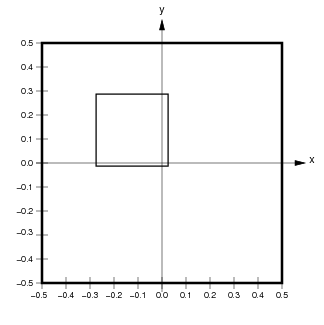
In addition to indexing (looking up a value), slicing (selecting a region) works as expected in continuous space (see the Indexing and Selecting user guide for more explanation). For instance, we can ask for a slice from (-0.275,-0.0125) to (0.025,0.2885) in continuous coordinates:
sl10=i10[-0.275:0.025,-0.0125:0.2885]
sl10.data
array([[-0.33, -0.23, -0.13],
       [-0.3 , -0.2 , -0.1 ],
       [-0.27, -0.17, -0.07]])
sl10
This slice has selected those array elements whose centers are contained within the specified continuous space. To do this, the continuous coordinates are first converted by HoloViews into the floating-point range (5.125,2.250) (2.125,5.250) of array coordinates, and all those elements whose centers are in that range are selected:
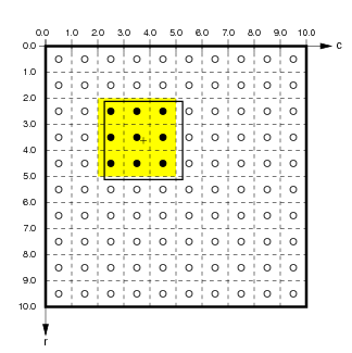 |
 |
Slicing also works for Raster elements, but it results in an object that always reflects the contents of the underlying Numpy array (i.e., always with the upper left corner labelled 0,0):
r5[0:3,1:3] + r5[0:3,1:2]
Hopefully these examples make it clear that if you are using data that is sampled from some underlying continuous system, you should use the continuous coordinates offered by HoloViews objects like Image so that your programs can be independent of the resolution or sampling density of that data, and so that your axes and indexes can be expressed naturally, using the actual units of the underlying continuous space. The data will still be stored in the same Numpy array, but now you can treat it consistently like the approximation to continuous values that it is.
1D and nD Continuous coordinates#
All of the above examples use the common case for visualizations of a two-dimensional regularly gridded continuous space, which is implemented in holoviews.core.sheetcoords.SheetCoordinateSystem.
Similar continuous coordinates and slicing are also supported for Chart elements, such as Curves, but using a single index and allowing arbitrary irregular spacing, implemented in holoviews.elements.chart.Chart.
They also work the same for the n-dimensional coordinates and slicing supported by the container types HoloMap, NdLayout, and NdOverlay, implemented in holoviews.core.dimension.Dimensioned and again allowing arbitrary irregular spacing.
QuadMesh elements are similar but allow more general types of mapping between the underlying array and the continuous space, with arbitrary spacing along each of the axes or even over the entire array. See the QuadMesh element for more details.
Together, these powerful continuous-coordinate indexing and slicing operations allow you to work naturally and simply in the full n-dimensional space that characterizes your data and parameter values.
Sampling#
The above examples focus on indexing and slicing, but as described in the Indexing and Selecting user guide there is another related operation supported for continuous spaces, called sampling. Sampling is similar to indexing and slicing, in that all of them can reduce the dimensionality of your data, but sampling is implemented in a general way that applies for any of the 1D, 2D, or nD datatypes. For instance, if we take our 10×10 array from above, we can ask for the value at a given location, which will come back as a Table, i.e. a dictionary with one (key,value) pair:
e10=i10.sample(x=-0.275, y=0.2885)
e10.opts(height=75)
Similarly, if we ask for the value of a given y location in continuous space, we will get a Curve with the array row closest to that y value in the Image 2D array returned as arrays of x values and the corresponding z value from the image:
r10=i10.sample(y=0.2885)
r10
The same sampling syntax can be used on HoloViews objects with any number of continuous-coordinate dimensions, in each case returning a HoloViews object of the correct dimensionality. This support for working in continuous spaces makes it much more natural to work with HoloViews objects than directly with the underlying raw Numpy arrays, but the raw data always remains available when needed.