Building Composite Objects#
The reference gallery shows examples of each of the container types in HoloViews. As you work through this guide, it will be useful to look at the description of each type there.
This guide shows you how to combine the various container types, in order to build data structures that can contain all of the data that you want to visualize or analyze, in an extremely flexible way. For instance, you may have a large set of measurements of different types of data (numerical, image, textual notations, etc.) from different experiments done on different days, with various different parameter values associated with each one. HoloViews can store all of this data together, which will allow you to select just the right bit of data “on the fly” for any particular analysis or visualization, by indexing, slicing, selecting, and sampling in this data structure.
Nesting hierarchy #
To illustrate the full functionality provided, we will create an example of the maximally nested object structure currently possible with HoloViews:
import numpy as np

import holoviews as hv

hv.extension('bokeh')
np.random.seed(10)

def sine_curve(phase, freq, amp, power, samples=102):
    xvals = [0.1* i for i in range(samples)]
    return [(x, amp*np.sin(phase+freq*x)**power) for x in xvals]

phases =      [0, np.pi/2, np.pi, 3*np.pi/2]
powers =      [1,2,3]
amplitudes =  [0.5,0.75, 1.0]
frequencies = [0.5, 0.75, 1.0, 1.25, 1.5, 1.75]


gridspace = hv.GridSpace(kdims=['Amplitude', 'Power'], group='Parameters', label='Sines')

for power in powers:
    for amplitude in amplitudes:
        holomap = hv.HoloMap(kdims='Frequency')
        for frequency in frequencies:
            sines = {phase : hv.Curve(sine_curve(phase, frequency, amplitude, power))
                     for phase in phases}
            ndoverlay = hv.NdOverlay(sines, kdims='Phase').relabel(group='Phases',
                                                                   label='Sines', depth=1)
            overlay = ndoverlay * hv.Points([(i,0) for i in range(10)], group='Markers', label='Dots')
            holomap[frequency] = overlay
        gridspace[amplitude, power] = holomap

penguins = hv.RGB.load_image('../reference/elements/assets/penguins.png').relabel(group="Family", label="Penguin")

layout = gridspace + penguins.opts(axiswise=True)


This code produces what looks like a relatively simple animation of two side-by-side figures, but is actually a deeply nested data structure:
layout
To help us understand this structure, here is a schematic for us to refer to as we unpack this object, level by level:
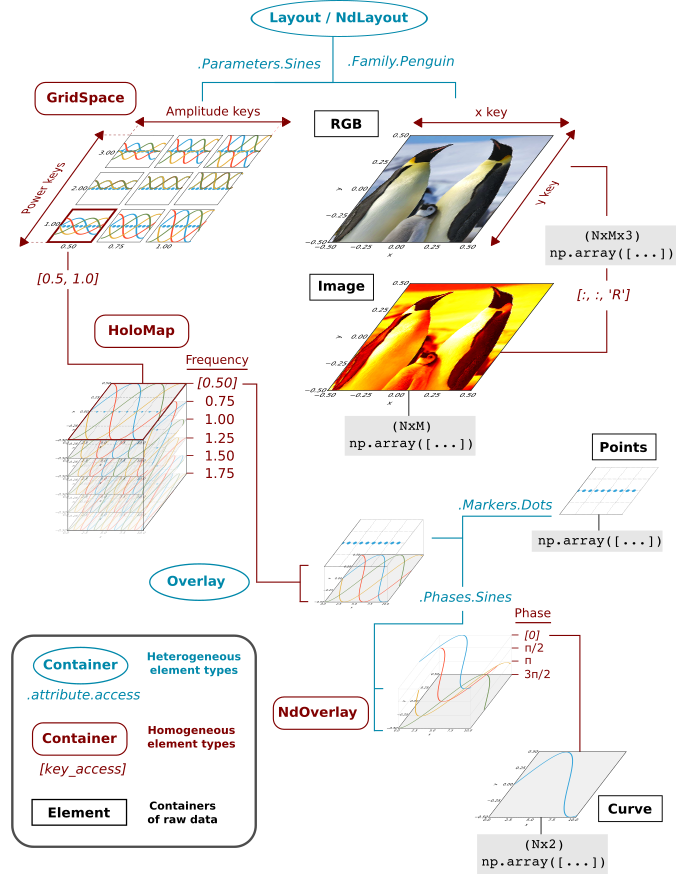
Everything that is displayable in HoloViews has this same basic hierarchical structure, although any of the levels can be omitted in simpler cases, and many different Element types (not containers) can be substituted for any other.
Since HoloViews 1.3.0, you are allowed to build data-structures that violate this hierarchy (e.g., you can put Layout objects into HoloMaps) but the resulting object cannot be displayed. Instead, you will be prompted with a message to call the collate method. Using the collate method will allow you to generate the appropriate object that correctly obeys the hierarchy shown above, so that it can be displayed.
As shown in the diagram, there are three different types of container involved:
Basic Element: elementary HoloViews object containing raw data in an external format like Numpy or pandas.
Homogeneous container (UniformNdMapping): collections of Elements or other HoloViews components that are all the same type. These are indexed using array-style key access with values sorted along some dimension(s), e.g.
[0.50]or["a",7.6].Heterogeneous container (AttrTree): collections of data of different types, e.g. different types of Element. These are accessed by categories using attributes, e.g.
.Parameters.Sines, which does not assume any ordering of a dimension.
We will now go through each of the containers of these different types, at each level.
Layout Level#
Above, we have already viewed the highest level of our data structure as a Layout. Here is the representation of the entire Layout object, which reflects all the levels shown in the diagram:
print(layout)
:Layout
   .Parameters.Sines :GridSpace   [Amplitude,Power]
      :HoloMap   [Frequency]
         :Overlay
            .Phases.Sines :NdOverlay   [Phase]
               :Curve   [x]   (y)
            .Markers.Dots :Points   [x,y]
   .Family.Penguin   :RGB   [x,y]   (R,G,B,A)
In the examples below, we will unpack this data structure using attribute access (explained in the Annotating Data user guide) as well as indexing and slicing (explained in the Indexing and Selecting Data user guide).
GridSpace Level#
Elements within a Layout, such as the GridSpace in this example, are reached via attribute access:
layout.Parameters.Sines
HoloMap Level#
This GridSpace consists of nine HoloMaps arranged in a two-dimensional space. Let’s now select one of these HoloMap objects by indexing to retrieve the one at [Amplitude,Power] [0.5,1.0], i.e. the lowest amplitude and power:
layout.Parameters.Sines[0.5, 1]
As shown in the schematic above, a HoloMap contains many elements with associated keys. In this example, these keys are indexed with a dimension Frequency, which is why the Frequency varies when you play the animation here.
Overlay Level#
The printed representation showed us that the HoloMap is composed of Overlay objects, six in this case (giving six frames to the animation above). Let us access one of these elements, i.e. one frame of the animation above, by indexing to retrieve an Overlay associated with the key with a Frequency of 1.0:
layout.Parameters.Sines[0.5, 1][1.0]
NdOverlay Level#
As the representation shows, the Overlay contains a Points object and an NdOverlay object. We can access either one of these using the attribute access supported by Overlay:
(layout.Parameters.Sines[0.5, 1][1].Phases.Sines +
 layout.Parameters.Sines[0.5, 1][1].Markers.Dots)
Curve Level#
The NdOverlay is so named because it is an overlay of items indexed by dimensions, unlike the regular attribute-access overlay types. In this case it is indexed by Phase, with four values. If we index to select one of these values, we will get an individual Curve, e.g. the one with zero phase:
l=layout.Parameters.Sines[0.5, 1][1].Phases.Sines[0.0]
l
print(l)
:Curve [x] (y)
Data Level#
At this point, we have reached the end of the HoloViews objects; below this object is only the raw data stored in one of the supported formats (e.g. NumPy arrays or Pandas DataFrames):
type(layout.Parameters.Sines[0.5, 1][1].Phases.Sines[0.0].data)
pandas.DataFrame
Actually, HoloViews will let you go even further down, accessing data inside the Numpy array using the continuous (floating-point) coordinate systems declared in HoloViews. E.g. here we can ask for a single datapoint, such as the value at x=5.2:
layout.Parameters.Sines[0.5, 1][1].Phases.Sines[0.0][5.2]
np.float64(-0.44172732786007657)
Indexing into 1D Elements like Curve and higher-dimensional but regularly gridded Elements like Image, Surface, and HeatMap will return the nearest defined value (i.e., the results “snap” to the nearest data item):
layout.Parameters.Sines[0.5, 1][1].Phases.Sines[0.0][5.23], layout.Parameters.Sines[0.5, 1][1].Phases.Sines[0.0][5.27]
(np.float64(-0.44172732786007657), np.float64(-0.4161337211119504))
For other Element types, such as Points, snapping is not supported and thus indexing down into the .data array will be less useful, because it will only succeed for a perfect floating-point match on the key dimensions. In those cases, you can still use all of the access methods provided by the numpy array itself, via .data, e.g. .data[52], but note that such native operations force you to use the native indexing scheme of the array, i.e. integer access starting at zero, not the more convenient and semantically meaningful continuous coordinate systems we provide through HoloViews.
Indexing using .select#
The curve displayed immediately above shows the final, deepest Element access possible in HoloViews for this object:
layout.Parameters.Sines[0.5, 1][1].Phases.Sines[0.0]
This is the curve with an amplitude of 0.5, raised to a power of 1.0 with frequency of 1.0 and 0 phase. These are all the numbers, in order, used in the access shown above.
The .select method is a more explicit way to use key access, with both of these equivalent to each other:
o1 = layout.Parameters.Sines.select(Amplitude=0.5, Power=1.0).select(Frequency=1.0)
o2 = layout.Parameters.Sines.select(Amplitude=0.5, Power=1.0, Frequency=1.0)
o1 + o2
The second form demonstrates HoloViews’ deep indexing feature, which allows indices to cross nested container boundaries. The above is as far as we can index before reaching a heterogeneous type (the Overlay), where we need to use attribute access. Here is the more explicit method of indexing down to a curve, using .select to specify dimensions by name instead of bracket-based indexing by position:
layout.Parameters.Sines.select(Amplitude=0.5,Power=1.0, Frequency=1.0, Phase=0.0).Phases.Sines
Summary#
As you can see, HoloViews lets you compose objects of heterogeneous types, and objects covering many different numerical or other dimensions, laying them out spatially, temporally, or overlaid. The resulting data structures are complex, but they are composed of simple elements with well-defined interactions, making it feasible to express nearly any relationship that will characterize your data. In practice, you will probably not need this many levels, but given this complete example, you should be able to construct an appropriate hierarchy for whatever type of data that you want to represent or visualize.
As emphasized above, it is not recommended to combine these objects in other orderings. Of course, any Element can be substituted for any other, which doesn’t change the structure. But you should not e.g. display an Overlay of Layout objects. The display system will generally attempt to figure out the correct arrangement and warn you to call the .collate method to reorganize the objects in the recommended format.
Another important thing to observe is that Layout and Overlay types may not be nested, e.g. using the + operator on two Layout objects will not create a nested Layout instead combining the contents of the two objects. The same applies to the * operator and combining of Overlay objects.